04: Linear Regression with Multiple Variables
Linear regression with multiple features
New version of linear regression with multiple features
- Multiple variables = multiple features
- In original version we had
- X = house size, use this to predict
- y = house price
- If in a new scheme we have more variables (such as number of bedrooms, number floors, age of the home)
- x1, x2, x3, x4 are the four features
- x1 - size (feet squared)
- x2 - Number of bedrooms
- x3 - Number of floors
- x4 - Age of home (years)
- y is the output variable (price)
- x1, x2, x3, x4 are the four features
- More notation
- n
- number of features (n = 4)
- m
- number of examples (i.e. number of rows in a table)
- xi
- vector of the input for an example (so a vector of the four parameters for the ith input example)
- i is an index into the training set
- So
- x is an n-dimensional feature vector
- x3 is, for example, the 3rd house, and contains the four features associated with that house
- xji
- The value of feature j in the ith training example
- So
- x23 is, for example, the number of bedrooms in the third house
- n
- Now we have multiple features
- What is the form of our hypothesis?
- Previously our hypothesis took the form;
- hθ(x) = θ0 + θ1x
- Here we have two parameters (theta 1 and theta 2) determined by our cost function
- One variable x
- hθ(x) = θ0 + θ1x
- Now we have multiple features
- hθ(x) = θ0 + θ1x1 + θ2x2 + θ3x3 + θ4x4
- For example
- hθ(x) = 80 + 0.1x1 + 0.01x2 + 3x3 - 2x4
- An example of a hypothesis which is trying to predict the price of a house
- Parameters are still determined through a cost function
- hθ(x) = 80 + 0.1x1 + 0.01x2 + 3x3 - 2x4
- For convenience of notation, x0 = 1
- For every example i you have an additional 0th feature for each example
- So now your feature vector is n + 1 dimensional feature vector indexed from 0
- This is a column vector called x
- Each example has a column vector associated with it
- So let's say we have a new example called "X"
- Parameters are also in a 0 indexed n+1 dimensional vector
- This is also a column vector called θ
- This vector is the same for each example
- Considering this, hypothesis can be written
- hθ(x) = θ0x0 + θ1x1 + θ2x2 + θ3x3 + θ4x4
- If we do
- hθ(x) =θT X
- θT is an [1 x n+1] matrix
- In other words, because θ is a column vector, the transposition operation transforms it into a row vector
- So before
- θ was a matrix [n + 1 x 1]
- Now
- θT is a matrix [1 x n+1]
- Which means the inner dimensions of θT and X match, so they can be multiplied together as
- [1 x n+1] * [n+1 x 1]
- = hθ(x)
- So, in other words, the transpose of our parameter vector * an input example X gives you a predicted hypothesis which is [1 x 1] dimensions (i.e. a single value)
- This x0 = 1 lets us write this like this
- hθ(x) =θT X
- This is an example of multivariate linear regression
Gradient descent for multiple variables
- Fitting parameters for the hypothesis with gradient descent
- Parameters are θ0 to θn
- Instead of thinking about this as n separate values, think about the parameters as a single vector (θ)
- Where θ is n+1 dimensional
- Our cost function is
- Similarly, instead of thinking of J as a function of the n+1 numbers, J() is just a function of the parameter vector
- J(θ)
- Gradient descent
simultaneously update for every j = 0, …, n
- Once again, this is
- θj = θj - learning rate (α) times the partial derivative of J(θ) with respect to θJ(...)
- We do this through a simultaneous update of every θj value
- Implementing this algorithm
- When n = 1
simultaneously update θ0 and θ1. The first update's sum is ∂/∂θ0 J(θ).
- Above, we have slightly different update rules for θ0 and θ1
- Actually they're the same, except the end has a previously undefined x0(i) as 1, so wasn't shown
- We now have an almost identical rule for multivariate gradient descent
simultaneously update θj for j = 0, …, n. The sum is ∂/∂θj J(θ).
import numpy as np

grad = X.T @ (X @ theta - y) / m   # every partial derivative at once
theta = theta - alpha * grad       # every parameter updated at once
The whole update rule in two lines: X.T @ (X @ theta − y) computes the sum in the equation above for every j simultaneously.
- What's going on here?
- We're doing this for each j (0 until n) as a simultaneous update (like when n = 1)
- So, we re-set θj to
- θj minus the learning rate (α) times the partial derivative of the θ vector with respect to θj
- In non-calculus words, this means that we do
- Learning rate
- Times 1/m (makes the maths easier)
- Times the sum of
- The hypothesis taking in the variable vector, minus the actual value, times the j-th value in that variable vector for EACH example
- It's important to remember that
- These algorithm are highly similar
Gradient Descent in practice: 1 Feature Scaling
- Having covered the theory, we now move on to learn about some of the practical tricks
- Feature scaling
- If you have a problem with multiple features
- You should make sure those features have a similar scale
- Means gradient descent will converge more quickly
- e.g.
- x1 = size (0 - 2000 feet)
- x2 = number of bedrooms (1-5)
- Means the contours generated if we plot θ1 vs. θ2 give a very tall and thin shape due to the huge range difference
- Running gradient descent on this kind of cost function can take a long time to find the global minimum
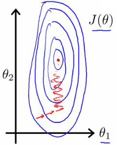
- Pathological input to gradient descent
- So we need to rescale this input so it's more effective
- So, if you define each value from x1 and x2 by dividing by the max for each feature
- Contours become more like circles (as scaled between 0 and 1)
- May want to get everything into -1 to +1 range (approximately)
- Want to avoid large ranges, small ranges or very different ranges from one another
- Rule of thumb regarding acceptable ranges
- -3 to +3 is generally fine - any bigger bad
- -1/3 to +1/3 is ok - any smaller bad
- Can do mean normalization
- Take a feature xi
- Replace it by (xi - mean)/max
- So your values all have an average of about 0
- Take a feature xi
μi is the average value of xi in the training set. si is the range (max − min), or the standard deviation.
mu = X[:, 1:].mean(axis=0)   # per-feature mean (skip the x0 column of 1s)
s  = X[:, 1:].std(axis=0)    # per-feature spread
X[:, 1:] = (X[:, 1:] - mu) / s   # every feature now centred, on a similar scale
Mean normalization and feature scaling in one step — broadcasting applies the subtraction and division to every row at once.
- Instead of max can also use standard deviation
Learning Rate α
- Focus on the learning rate (α)
- Topics
- Update rule
- Debugging
- How to choose α
Make sure gradient descent is working
-
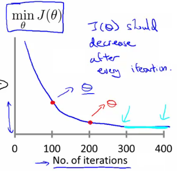
Plot min J(θ) vs. no of iterations
- (i.e. plotting J(θ) over the course of gradient descent
- If gradient descent is working then J(θ) should decrease after every iteration
-
Can also show if you're not making huge gains after a certain number
- Can apply heuristics to reduce number of iterations if need be
- If, for example, after 1000 iterations you reduce the parameters by nearly nothing you could choose to only run 1000 iterations in the future
- Make sure you don't accidentally hard-code thresholds like this in and then forget about why they're there though!
-
Number of iterations varies a lot
- 30 iterations
- 3000 iterations
- 3,000,000 iterations
- Very hard to tell in advance how many iterations will be needed
- Can often make a guess based a plot like this after the first 100 or so iterations
-
Automatic convergence tests
-
Check if J(θ) changes by a small threshold or less
- Choosing this threshold is hard
-
So often easier to check for a straight line
- Why? - Because we're seeing the straightness in the context of the whole algorithm
- Could you design an automatic checker which calculates a threshold based on the system's preceding progress?
-
Check if J(θ) changes by a small threshold or less
-
Checking it's working
-
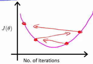
If you plot J(θ) vs iterations and see the value is increasing - means you probably need a smaller α
- Cause is because you're minimizing a function which looks like this
-
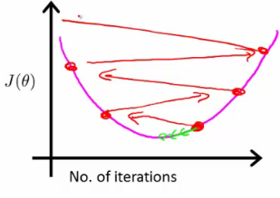
If you plot J(θ) vs iterations and see the value is increasing - means you probably need a smaller α
- But you overshoot, so reduce learning rate so you actually reach the minimum (green line)
- So, use a smaller α
-
Another problem might be if J(θ) looks like a series of waves
- Here again, you need a smaller α
-
However
- If α is small enough, J(θ) will decrease on every iteration
-
BUT, if α is too small then rate is too slow
- A less steep incline is indicative of a slow convergence, because we're decreasing by less on each iteration than a steeper slope
-
Typically
- Try a range of alpha values
- Plot J(θ) vs number of iterations for each version of alpha
-
Go for roughly threefold increases
- 0.001, 0.003, 0.01, 0.03. 0.1, 0.3
Features and polynomial regression
- Choice of features and how you can get different learning algorithms by choosing appropriate features
- Polynomial regression for non-linear function
- Example
- House price prediction
- Two features
- Frontage - width of the plot of land along road (x1)
- Depth - depth away from road (x2)
- Two features
- You don't have to use just two features
- Can create new features
- Might decide that an important feature is the land area
- So, create a new feature = frontage * depth (x3)
- h(x) = θ0 + θ1x3
- Area is a better indicator
- Often, by defining new features you may get a better model
- House price prediction
- Polynomial regression
- May fit the data better
- θ0 + θ1x + θ2x2 e.g. here we have a quadratic function
- For housing data could use a quadratic function
- But may not fit the data so well - inflection point means housing prices decrease when size gets really big
- So instead must use a cubic function
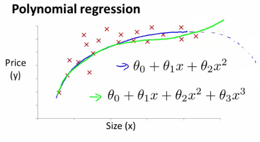
- How do we fit the model to this data
- To map our old linear hypothesis and cost functions to these polynomial descriptions the easy thing to do is set
- x1 = x
- x2 = x2
- x3 = x3
- By selecting the features like this and applying the linear regression algorithms you can do polynomial linear regression
- Remember, feature scaling becomes even more important here
- To map our old linear hypothesis and cost functions to these polynomial descriptions the easy thing to do is set
- Instead of a conventional polynomial you could do variable ^(1/something) - i.e. square root, cubed root etc
- Lots of features - later look at developing an algorithm to choose the best features
Normal equation
- For some linear regression problems the normal equation provides a better solution
- So far we've been using gradient descent
- Iterative algorithm which takes steps to converge
- Normal equation solves θ analytically
- Solve for the optimum value of theta
- Has some advantages and disadvantages
How does it work?
- Simplified cost function
- J(θ) = aθ2 + bθ + c
- θ is just a real number, not a vector
- Cost function is a quadratic function
- How do you minimize this?
- Do
- Take derivative of J(θ) with respect to θ
- Set that derivative equal to 0
- Allows you to solve for the value of θ which minimizes J(θ)
- Do
- J(θ) = aθ2 + bθ + c
- In our more complex problems;
- Here θ is an n+1 dimensional vector of real numbers
- Cost function is a function of the vector value
- How do we minimize this function
- Take the partial derivative of J(θ) with respect to θj and set to 0 for every j
- Do that and solve for θ0 to θn
- This would give the values of θ which minimize J(θ)
- How do we minimize this function
- If you work through the calculus and the solution, the derivation is pretty complex
- Not going to go through here
- Instead, what do you need to know to implement this process
Example of normal equation
| Size in feet2 (x1) | Number of bedrooms (x2) | Number of floors (x3) | Age of home in years (x4) | Price ($1000) (y) |
|---|---|---|---|---|
| 2104 | 5 | 1 | 45 | 460 |
| 1416 | 3 | 2 | 40 | 232 |
| 1534 | 3 | 2 | 30 | 315 |
| 852 | 2 | 1 | 36 | 178 |
- Here
- m = 4
- n = 4
- To implement the normal equation
- Take examples
- Add an extra column (x0 feature)
- Construct a matrix (X - the design matrix) which contains all the training data features in an [m x n+1] matrix
- Do something similar for y
- Construct a column vector y vector [m x 1] matrix
- Using the following equation (X transpose * X) inverse times X transpose y
That is XTX inverted, times XT, times y — the normal equation with the table above substituted in.
X = np.array([[1, 2104, 5, 1, 45],
              [1, 1416, 3, 2, 40],
              [1, 1534, 3, 2, 30],
              [1,  852, 2, 1, 36]], dtype=float)
y = np.array([460, 232, 315, 178], dtype=float)

theta = np.linalg.pinv(X.T @ X) @ X.T @ y

X @ theta   # [460., 232., 315., 178.]  -> reproduces every price exactly
The table above, solved in one line. With only four examples and five parameters the fit is exact — X @ theta returns the y column to machine precision.
- If you compute this, you get the value of theta which minimize the cost function
General case
- Have m training examples and n features
- The design matrix (X)
- Each training example is a n+1 dimensional feature column vector
- X is constructed by taking each training example, determining its transpose (i.e. column -> row) and using it for a row in the design matrix
- This creates an [m x (n+1)] matrix
Each training example is a column vector; its transpose becomes one row of the design matrix, giving an [m x (n+1)] matrix.
- Vector y
- Used by taking all the y values into a column vector
- The design matrix (X)
- What is this equation?!
- (XT * X)-1
- What is this --> the inverse of the matrix (XT * X)
- i.e. A = XT X
- A-1 = (XT X)-1
- What is this --> the inverse of the matrix (XT * X)
- (XT * X)-1
- In Python you could do;
theta = np.linalg.pinv(X.T @ X) @ X.T @ y
- X.T is the notation for X transpose
- np.linalg.pinv is a function for the (pseudo) inverse of a matrix
- In a previous lecture discussed feature scaling
- If you're using the normal equation then no need for feature scaling
When should you use gradient descent and when should you use the normal equation?
- Gradient descent
- Need to choose learning rate
- Needs many iterations - could make it slower
- Works well even when n is massive (millions)
- Better suited to big data
- What is a big n though
- 100 or even a 1000 is still (relatively) small
- If n is 10 000 then look at using gradient descent
- Normal equation
- No need to choose a learning rate
- No need to iterate, check for convergence etc.
- Normal equation needs to compute (XT X)-1
- This is the inverse of an n x n matrix
- With most implementations computing a matrix inverse grows by O(n3 )
- So not great
- Slow if n is large
- Can be much slower
Normal equation and non-invertibility
- Advanced concept
- Often asked about, but quite advanced, perhaps optional material
- Phenomenon worth understanding, but not probably necessary
- When computing (XT X)-1 * XT * y)
- What if (XT X) is non-invertible (singular/degenerate)
- Only some matrices are invertible
- This should be quite a rare problem
- NumPy can invert matrices using
- np.linalg.pinv (pseudo inverse)
- This gets the right value even if (XT X) is non-invertible
- np.linalg.inv (inverse)
- np.linalg.pinv (pseudo inverse)
- NumPy can invert matrices using
- What does it mean for (XT X) to be non-invertible
- Normally two common causes
- Redundant features in learning model
- e.g.
- x1 = size in feet
- x2 = size in meters squared
- e.g.
- Too many features
- e.g. m <= n (n is much larger than m)
- m = 10
- n = 100
- Trying to fit 101 parameters from 10 training examples
- Sometimes work, but not always a good idea
- Not enough data
- Later look at why this may be too little data
- To solve this we
- Delete features
- Use regularization (lets you use lots of features for a small training set)
- e.g. m <= n (n is much larger than m)
- Redundant features in learning model
- Normally two common causes
- If you find (XT X) to be non-invertible
- Look at features --> are features linearly dependent?
- So just delete one, will solve problem
- Look at features --> are features linearly dependent?
- What if (XT X) is non-invertible (singular/degenerate)